ORIGIN

EEG and EMG Data Processing (Matlab)

2025-01-17

EEGEMG EEG EMG Matlab EEGLAB 15 mins2.4k words

This article introduces the preprocessing of EEG and EMG data. The goal is to analyze the correlation between EEG and EMG data on the same timescale, and the raw data collected is in TXT format with EEG and EMG data stored together. You can directly use the graphical interface here: Github Repo: EEG_EMG Process

This article covers the processing of single data. If you use my graphical UI interface, you can process data in batches. It will automatically read data from files for processing.

Data Format Overview

Before preprocessing the EEG data, understanding the basic format of the data is crucial. Below is an example of the format of the collected EEG and EMG data:

# MIX|None|0+True+胫骨前肌+1000|1+True+腓骨长肌+1000|2+True+腓肠肌内侧+1000|3+True+腓肠肌外侧+1000|4+True+股直肌+1000|5+True+股内侧肌+1000|6+True+股二头肌长头+1000|7+True+半腱肌+1000|8+False+胫骨前肌+1000|9+False+腓骨长肌+1000|10+False+肠肌内侧+1000|11+False+肠肌外侧+1000|12+False+EMG13+1000|13+False+EMG14+1000|14+False+EMG15+1000|15+False+EMG16+1000|0+True+P4+80|1+True+CP2+80|2+True+FC5+80|3+True+C3+80|4+True+P3+80|5+True+C2+80|6+True+FC6+80|7+True+C4+80|8+True+CP6+80|9+True+F3+80|10+True+FC2+80|11+True+FC1+80|12+True+F4+80|13+True+CP5+80|14+True+C1+80|15+True+CP1+80
# 13425+24732+39459+51551+66531+77703+93361+104448+119984+130913+145827+157066
0.00    0.00    0.00    0.00    0.00    0.00    0.00    0.00    0.00    0.00    0.00    0.00    0.00    0.00    0.00    0.00    0.00    0.00    0.00    0.00    0.00    0.00    0.00    0.00    0.00    0.00    0.00    0.00    0.00    0.00    0.00    0.00
...

Data Format Description

Header:
- MIX|None|: Describes the data type (e.g., MIX could be mixed signals).
- X+True/False+Channel+SampleRate: Represents information about different channels, including whether they are enabled (True/False), the channel name (e.g., Tibialis Anterior, P4, etc.), and the sampling rate (in Hz).
Marker Information: Timepoint data starting with #, such as 13425+24732+39459.... This represents marker data from the experiment. However, in this experiment, markers are not used due to inaccuracies.
Signal Data: Each line represents the signal values at a specific time point, with columns corresponding to different channels.

Data Preparation

Data Filtering

If you use my graphical interface for processing, you don’t need to worry about this step—it will be done automatically.

Read Data from File

First, use MATLAB to read the raw data from the file with the following code:

1
2
3

fid = fopen(filepath);
% ... verify fid
datafile = textscan(fid, repmat('%f', 1, 32), 'Delimiter', '\t', 'CommentStyle', '#');

Extract EEG, EMG

Based on the experimental requirements, extract the EEG and EMG data. EMG is from columns 1-8, and EEG is from columns 17-32.

1 2	EMGData = [datafile{1:8}]; EEGData = [datafile{17:32}];

Filtering Process

EEG Signal: Focuses on the 1-49 Hz frequency range, which contains most of the brainwave activity, such as alpha and beta waves. Eliminate 50 Hz power line interference.
EMG Signal: Focuses on the 20-150 Hz frequency range, which contains the main features of the electromyogram. Also eliminate 50 Hz interference.

function [EMGData, EEGData] = filterData(EMGData, EEGData)
    fs = 1000; % Sampling frequency

    % Power line interference filter: 50 Hz and its harmonics
    for j = 1:9
        [b, a] = butter(2, [2*(50*j-1)/fs, 2*(50*j+1)/fs], "stop");
        EMGData = filter(b, a, EMGData);
        EEGData = filter(b, a, EEGData);
    end

    % Band-pass filter: Extract relevant frequency ranges
    % EMG 20-150 Hz
    [b, a] = butter(4, [2*20/fs, 2*150/fs], "bandpass");
    EMGData = filter(b, a, EMGData);

    % EEG 1-49 Hz
    [b, a] = butter(4, [2*1/fs, 2*49/fs], "bandpass");
    EEGData = filter(b, a, EEGData);
end

Manual Correction of Markers

Due to missing or inaccurate marker information, you need to manually correct the marker data. First, plot the data and find the precise positions from the graph.

N1 = length(EMGData(1,:)); % Number of EMG channels
N2 = length(EEGData(1,:)); % Number of EEG channels
N = N1 + N2; % Total number of channels (24 channels corresponding to the 24 channels in eegemg_sitstand_locs.ced file)

if isempty(findall(0, 'Name', ['Window ' char(filename)], 'Type', 'figure'))
    hFig = figure;  % Create a new window if not found
    disp("Didn't find existing window, create a new one")
else
    hFig = findall(0, 'Name', ['Window ' char(filename)], 'Type', 'figure');
    close(hFig);  % Close any existing figure
    hFig = figure;  % Create a new figure
end

% Data Display - excluding certain EMG channels
yrangeEMG = 200;
yrangeEEG = 100;
t = 0.001:0.001:length(EMGData(:,1))/1000; % Time vector in seconds
offsets = zeros(N, 1); % Create an offset matrix initialized with zeros

set(gcf, 'Name', ['Window ' char(filename)]);
hold on
for j=1:8
    if ismember(j, EMGBanList)
        result = 0;
    else
        result = 1;
    end
    offsets(j) = yrangeEMG*(N1-j);
    plot(t, (EMGData(:,j)+offsets(j))*result)
end
for j=1:16
    if ismember(j, EEGBanList)
        result = 0;
    else
        result = 1;
    end
    offsets(N1+j) = yrangeEMG*(N1)+200+yrangeEEG*(16-j);
    plot(t, (EEGData(:,j)+offsets(N1+j))*result)
end

hold off
channelLabels = {'TA','PL','MG','LG','RF','VM','LBF','Semi', 'P4','CP2','FC5','C3','P3','C2','FC6','C4','CP6','F3

You can manually recover the original positions after obtaining the dotting information, or store them separately.

Generating Event Information

You need to manually construct the event information file.

File Format Requirements

Event information files must use plain text format (.txt), where each line represents a single event record, and fields are separated by spaces, commas, or tabs. It is recommended to use tab-separated (tab-separated values) for easy parsing.

Required Fields and Descriptions

Field Name	Data Type	Required	Description
`type`	String	Yes	Event type identifier, e.g., `'Stimulus'` or `'Response'`.
`latency`	Numeric	Yes	The sampling point of the event in the EEG data (in samples).
`duration`	Numeric	No	Duration of the event in samples, fill with `0` if unknown.
`epoch`	Numeric	No	The segment number, required only when EEG data is segmented.
`urevent`	Numeric	No	The event number linked to the original event data for traceability.

Example Content (TXT Format)

The file can be stored simply as events.txt, for example:

type    latency duration
a        512     100
b        1024    50
a        2048    100

Data Cutting

At this step, cut the data based on the dotting information and the duration of each event, leaving only the useful parts.

Using EEGLAB for Processing

Data Import (`set`)

1 2	EEG = pop_importdata('dataformat','ascii','nbchan',0,'data',filepath,'setname',eventFileName,'srate',1000,'pnts',0,'xmin',0,'chanlocs',locs_path); pop_importdata

This is one of the core functions in EEGLAB for importing raw data.
It allows importing multiple formats (e.g., ASCII, MATLAB variables) and setting key parameters (like sampling rate and number of channels).

Parameter Explanation:

Parameter	Example Value	Description
`dataformat`	`'ascii'`	Data format type; `'ascii'` means the data is stored in text format, other values can be `'matlab'` or native formats.
`nbchan`	`0`	Number of channels in the data, `0` means auto-detect the number of channels (common), or you can specify the actual count.
`data`	`filepath`	Path to the data file, which contains actual signal data; each row represents a time point, and columns represent channel data.
`setname`	`eventFileName`	Name of the dataset that will appear in the EEGLAB graphical interface, used to identify the imported EEG dataset.
`srate`	`1000`	Sampling rate of the data in Hz. For example, `1000` means 1000 samples per second.
`pnts`	`0`	Number of samples per channel, `0` means auto-detected from the file.
`xmin`	`0`	The start time of the data (in seconds); `0` means from the first sample point.
`chanlocs`	`locs_path`	The path to the channel location information file, typically `.loc` or `.ced` files, which define the spatial locations (electrode positions).

My chanlocs file looks like this:

Number	labels	theta	radius	X	Y	Z	sph_theta	sph_phi	sph_radius	type	
1	TA	   	   	   	   	   	   	   	   	EMG	
2	PL	   	   	   	   	   	   	   	   	EMG	
3	MG	   	   	   	   	   	   	   	   	EMG	
4	LG	   	   	   	   	   	   	   	   	EMG	
5	RF	   	   	   	   	   	   	   	   	EMG	
6	VM	   	   	   	   	   	   	   	   	EMG	
7	LBF	   	   	   	   	   	   	   	   	EMG	
8	SEM	   	   	   	   	   	   	   	   	EMG	
9	P4	145	0.331	-78.6	-55.7	56.6	-145	30.4	112	EEG	
10	CP2	141	0.188	-47.1	-38.4	90.7	-141	56.2	109	EEG	
11	FC5	-76.4	0.405	18.6	77.2	24.5	76.4	17.1	83.1	EEG	
12	C3	-100	0.255	-11.6	65.4	64.4	100	44.1	92.5	EEG	
13	P3	-146	0.331	-78.8	 53	55.9	146	30.5	110	EEG	
14	C2	104	0.132	-9.62	-37.7	88.4	-104	66.3	96.6	EEG	
15	FC6	75.9	0.408	19.9	-79.5	24.4	-75.9	16.6	85.6	EEG	
16	C4	99.2	0.261	-10.9	-67.1	63.6	-99.2	43.1	93.1	EEG	
17	CP6	119	0.399	-46.1	-83.3	31.2	-119	18.1	100	EEG	
18	F3	-43.4	0.333	53.1	50.2	42.2	43.4	 30	84.4	EEG	
19	FC2	52.8	0.161	26.4	-34.8	78.8	-52.8	 61	90.1	EEG	
20	FC1	-52.6	0.157	 26	34.1	 80	52.6	61.8	90.7	EEG	
21	F4	43.7	0.341	54.3	-51.8	40.8	-43.7	28.5	85.5	EEG	
22	CP5	-120	0.397	-46.6	79.6	30.9	120	18.6	97.3	EEG	
23	C1	-105	0.126	-9.98	36.2	89.8	105	67.3	97.3	EEG	
24	CP1	-143	0.183	-47.3	35.5	91.3	143	57.1	109	EEG

Note: The original file did not look like this. However, when directly importing raw EEG, the position may rotate 90 degrees, leading to an error. It requires manual correction each time the data is imported, or once the positions are fixed, export the corrected map and store it for future use.

Bad Channel Interpolation

Plotting Waveform

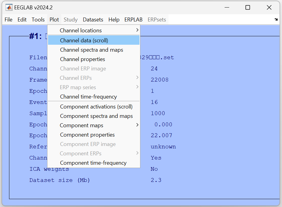
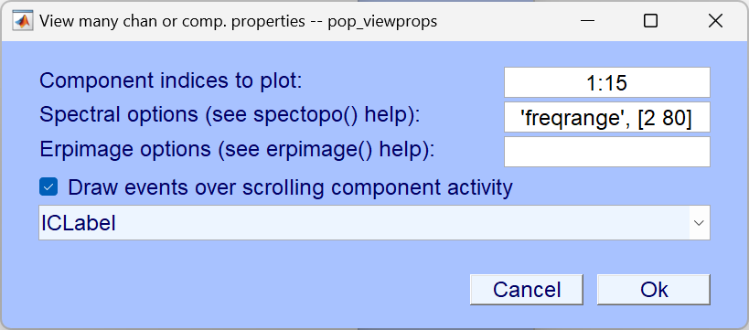
Use the built-in EEGLAB function pop_eegplot to draw EEG waveform graphs.

1	pop_eegplot(EEG, 1, 1, 0); % Draw the waveform for the data

Parameter Explanation:

EEG: The EEGLAB data structure, containing the imported data.
1 (continuous signal mode): Plot the raw continuous signal.
1 (channel index label): Display channel labels on the plot.
0 (single window): Display all channels in a single window; 1 would show each channel in a separate window.

Plotting via the graphical interface

Identifying Bad Channels

Based on the waveform plot, determine which channels are corrupted by checking:

Signal Anomalies:

Flat signal: A channel data is just a flat line, indicating the sensor may have disconnected or the signal was lost.
Abnormal high amplitude: If a channel shows consistently higher amplitude than others, this could indicate a poor connection or equipment issue.
High-frequency noise: If a channel shows irregular high-frequency signals, this could indicate technical issues.

Spatial Inconsistency:

Check the head map for the electrode distribution. A damaged channel may appear isolated on the map with abnormal signal spikes/drops in contrast to neighboring channels.

Interpolating Bad Channels

Use code for interpolation:

1	EEG_interp = pop_interp(EEG, selectedIndices, 'spherical')

Parameter Explanation:

EEG: The original EEG data structure.
selectedIndices: An array of indices for channels requiring interpolation.
'spherical': The interpolation method. This spherical interpolation takes into account the three-dimensional spatial arrangement of electrodes on a sphere, which is appropriate for EEG data.

Manual Interpolation

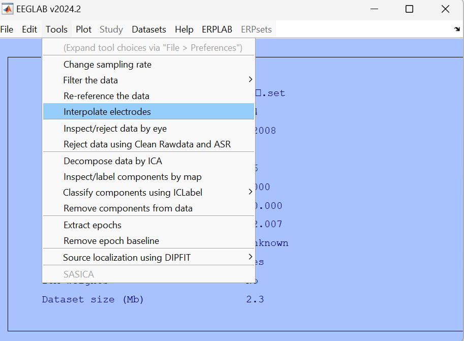
Select the channels that need interpolation.

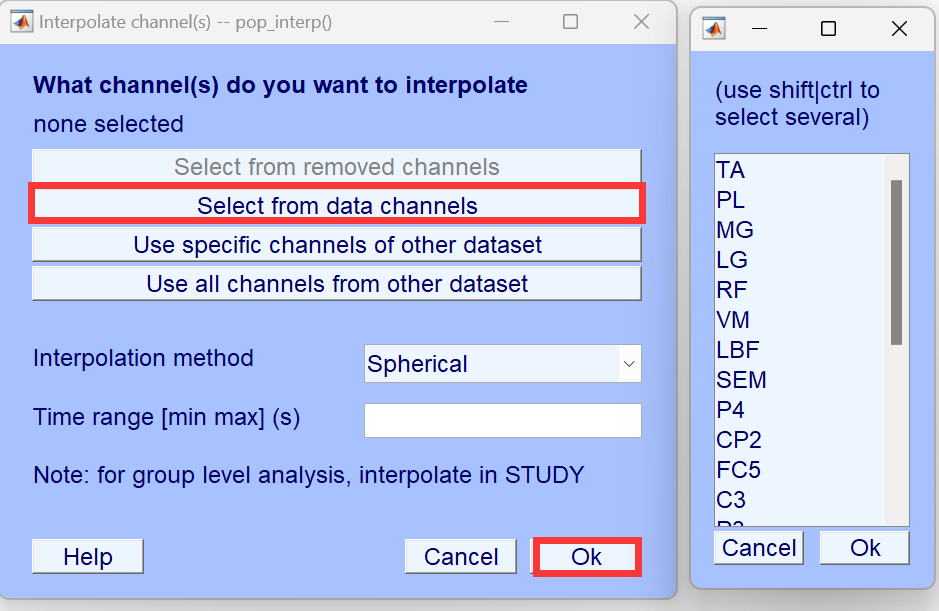
Note: Interpolation must be done for all channels at once, and cannot be performed in multiple steps.

Removing Artifacts and Noise

Independent Component Analysis (ICA)

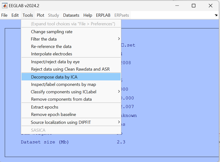
To remove artifacts such as eye movements or muscle activities, use ICA:

1	EEG = pop_runica(EEG, 'icatype', 'runica', 'extended', 1, 'interrupt', 'on', 'chanind', EEG_chans, 'pca', restLen);

Parameter Explanation:

icatype, runica: The ICA algorithm to be used (RunICA).
extended, 1: Use extended mode, which adds dimensionality to the analysis, suitable for multichannel data.
interrupt, on: Allow interruption during ICA computation.
chanind, EEG_chans: Indices of EEG channels that will participate in ICA (since EEG and EMG data are together, we should select the EEG channels).
pca, restLen: Using PCA to reduce the data’s dimensions. restLen represents the number of principal components (EEG electrode count - interpolated bad channel count).

This step aims to extract independent components from EEG data to eliminate artifacts while retaining components that reflect neural activity.

Or you can use the manual approach.

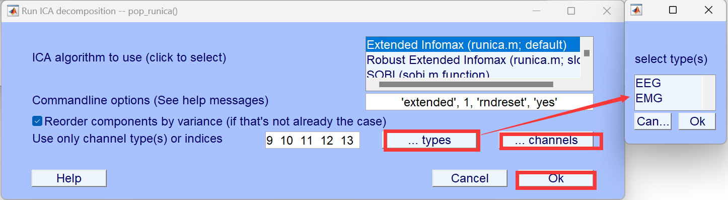
The data selection can be done in two ways, assuming categories for channels are already labeled.

During the execution, windows can pop up for real-time interruptions if necessary.

Mark Artifacts

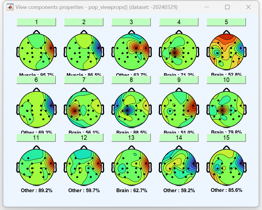
You can mark the data with labels, tagging artifacts as necessary:

EEG_temp = EEG;  % 
EEG_temp = pop_icflag(EEG_temp, [
    0.2 0.6;   % Brain: Brain activity components
    0.1 0.8;   % Muscle: Electromyographic artifacts
    0.2 0.7;   % Eye: Eye movement artifacts
    0.3 0.7;   % Heart: Electrocardiographic artifacts
    0.4 0.6;   % Line Noise: Power line noise
    0.1 0.9;   % Channel Noise: Channel signal noise
    0.0 0.9    % Other: Other artifacts
]);

Manual execution: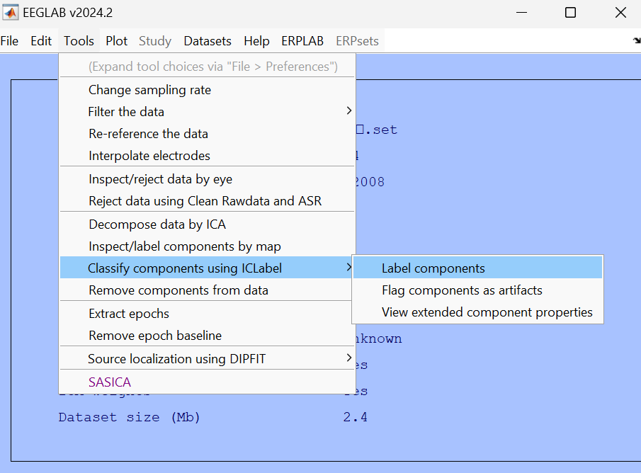

After marking, the flagged content will pop up. This image doesn’t serve any particular purpose and can be closed directly; it’s the classification drawn after automatic artifact analysis.

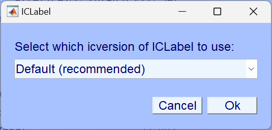
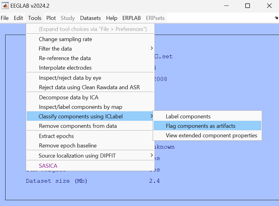
Then use the "flag components as artifact" function to automatically mark the artifacts.

Set thresholds for different categories.

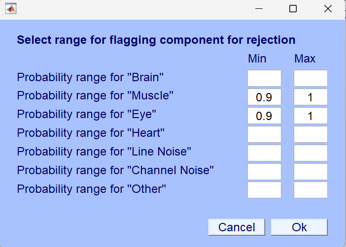Set the required thresholds based on your data. For my own data, I set the threshold for each category to 0.55, because my data has many interference factors.

Delete artifacts

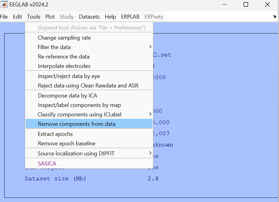
1 2	rejected_comps = find(EEG_temp.reject.gcompreject > 0); EEG_temp = pop_subcomp(EEG_temp, rejected_comps);

At this point, all data processing has been completed.

Author: o_oyao

Link: http://dyingdown.github.io/2025/01/17/EEG-and-EMG-Data-Processing-Matlab/

License: All articles in this blog are licensed under CC BY-NC-SA 4.0 unless stating additionally.

TOP

COMMENT

ABOUT
|
DONATE

o_oyao

The Jigsaw puzzle is incomplete with even one missing piece. And I want to be the last piece to make the puzzle complete.

Like my post?

EEG and EMG Data Processing (Matlab)

Data Format Overview

Data Format Description

Data Preparation

Data Filtering

Read Data from File

Extract EEG, EMG

Filtering Process

Manual Correction of Markers

Generating Event Information

File Format Requirements

Required Fields and Descriptions

Example Content (TXT Format)

Data Cutting

Using EEGLAB for Processing

Data Import (set)

Bad Channel Interpolation

Plotting Waveform

Parameter Explanation:

Identifying Bad Channels

Interpolating Bad Channels

Removing Artifacts and Noise

Independent Component Analysis (ICA)

Mark Artifacts

Delete artifacts

Data Import (`set`)